Tutorial 4: Exploratory analysis

Now that we have completed the tutorials on data handling, it is finally time to do some data analysis! In this tutorial, we will focus on the same data set by Qian et al that we used in the last tutorials. We will use plankton’s unsupervized spatial embedding routine to determine tissue structures and visualize spatio-topographical relationships in a number of scatter plots.

Recurring spatial contexts

Plankton uses the powerful UMAP embedding algorithm to retrieve recorring spatial contexts in the molecular topography. To this end, an individual model of the immediate environment is created per molecule spot. A KNN graph is generated around each spot and the distance-weighted counts of genes is stored as a vector. UMAP uses these vectors to create an easy to visualize 2d embedding.

To be able to run this tutorial, open the notebook tutorials/exploratory.ipynb, run the first cells to load the data set and initialize an sdata object:

sdata = pl.SpatialData(
                  x_coordinates=spot_data.x,
                  y_coordinates=spot_data.y,
                  genes=spot_data.Gene,
                  )

All graph-based analysis takes place in the sdata.graph object, that contains a k-nearest-neighbor graph and a few convenience functions for graph-based topographical analysis and visualization.

To update the interal knn graph, run the function:

sdata.graph.update_knn(n_neighbors=200)

This function calculates a 200-nearest neighbor graph and stores the data in the sdata.graph object. For our particular use case, the number of neighbors should be large enough to create a representative model of the local environment. In general, the larger the knn graph, the better - within the limits of your computational resources.

Now, we can create local environment models and run the UMAP algorithm:

#environment model building parameters:
bandwidth   = 60 #bandwidth of distance weight discount effect
zero_weight = 1  #regularization parameter

#UMAP parameters:
n_neighbors = 30
min_dist    = 0.03

sdata.graph.run_umap(
            bandwidth=bandwidth,
            zero_weight=zero_weight
            n_neighbors=n_neighbors,
            min_dist=min_dist,)

The function should complete within a couple of minutes. It creates a 2d array of embedding coordinates and stores it in sdata.graph.umap.

We can inspect the generated embedding using the function umap_paired:

sdata.graph.map_and_umap(marker='x',alpha=0.5)

Both the tissue map on the left and the embedding on the eight show molecules colored by gene label. We can already vaguely discern three main structures in the embedding:

• A compact, light-green cluster at the top

• a compact, green-blue cluster in the middle, and

• an elongated, dark-green structure at the bottom.

All in all, the above representation is most suitable for plotting, where the parameters can be changed using the generic matplotlib arguments and syntax. For a more interactive approach, plankton offers a javascript-based data viewer with a similar layout. It is created as follows:

sdata.graph.umap_js()

It also shows a scatter point map representation of the sdata coordinates on the left and the umap embedding on the right. Both maps offer a number of tool that help investigating the data, such as zooming and panning. The interface also offers lassoo and box selecton tools that can be used to select data points in either of the two panels, with the selected molecules being highlighted in both panels. Bar charts on the bottom show the most abundant molecules in the selection. Try to play around with the data to find topographical expression patterns.

When highlighted in the js viewer, the above-mentioned cluster structures seem to indeed represent spatially coherent tissue regions. In the next step, we want to store these regions for further plotting and statistical investigation.

To do this, select the central cluster (like in the screen capture above), type the name ‘radiatum’ into the Name text field and hit the store selection button. The js viewer now added the selection as a boolean column to our sdata data frame:

	g	x	y	gene_id	radiatum
0	Cxcl14	110	5457	24	False
1	Plp1	-1	4735	56	False
2	Plp1	-1	4725	56	False
3	Id2	-1	4478	35	False
4	Enpp2	-1	4455	26	False
...	...	...	...	...	...
72331	Npy	7305	1257	45	False
72332	Npy	7331	1360	45	False
72333	Npy	7425	1294	45	False
72334	Npy	7467	1287	45	False
72335	Npy	7492	1268	45	False

72336 rows × 5 columns

This boolean column denotes category membership and can be used for plotting color assignment or dataset subselecting:

sdata_radiatum = sdata[sdata.radiatum]

sdata_radiatum

	g	x	y	gene_id	radiatum
1169	Nrn1	204	4448	48	True
1173	Nrn1	205	4458	48	True
1174	Nrn1	205	4449	48	True
1187	Nrn1	210	4453	48	True
1202	Id2	214	4323	35	True
...	...	...	...	...	...
72138	Npy	5985	1343	45	True
72140	Npy	5991	1348	45	True
72142	Npy	6002	1357	45	True
72164	Npy	6243	1550	45	True
72174	Npy	6324	1634	45	True

The idea for the rest of this tutorial is to plot the three subsections on top of each other, each with a different colormap, to visualize the spatial relations within and across the detected clusters. To this end, please:

• Select the topmost,light-green cluster and give it the name ‘alveus’

• Through selection (or using boolean logic with the other two clusters) store the large, elongated structure in the column ‘pyramidal’.

• Just like sdata_radiatum above, create two new sdata sets sdata_alveus and sdata_pyramidal.

The UMAP output coordnates are stored as an n . 2 array under sdata.graph.umap. X-coordinates are stored in the first column, y-coordinates in the second.

The coodinate subsets can now be plotted using sdata.scatter and sdata.graph.plot_umap() with the respective arguments for c and cmap:

#extract umap's y-coordinates:
umap_y = sdata_radiatum.graph.umap[:,1]

#plot umap with color grading:
sdata_radiatum.graph.plot_umap(c=umap_y
                        cmap='autumn')

#plot umap-y in tissue coordinates
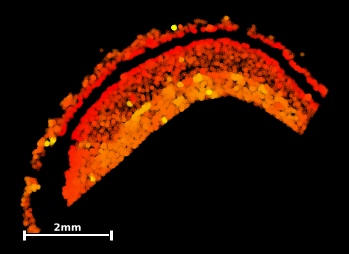
sdata_radiatum.scatter(c=umap_y
                        cmap='autumn')

This exploratory result provides us with a few hypotheses that we could test during further analysis:

• The stratum radiatum is detected as two distinct and connected structures around a central gap.

• The main topographical feature determining local molecular composition appears to be the proximity to the central gap, with gap-proximal molecules being displayed in the southernmost part of the UMAP.

• A few outliers (bright yellow) do seem to embedded in the radiatum matrix but form islets with a distinct molecular composition of their own.

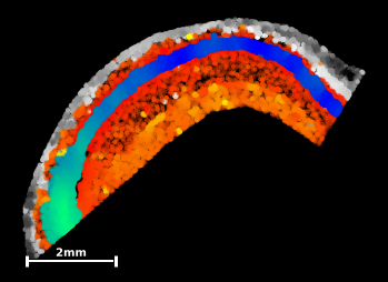
In the next step, add scatterplots of the other two data subsets to the output figure, giving ‘alveus’ a y-axis gradient with the colormap ‘Greys’, and ‘pyramidal’ an x-axis gradient with the colormap ‘winter’ (you can remove unnecessary scalebars through the argument scalebar=False).

The final output should look something like this:

Aren’t we lucky to work in such a visually appealing field : ) Our whole-genome-sequencing friends might have a harder time producing pretty pictures like this…

But this output also gives us a few more observatons that could be tested in upstream analysis:

• The pyramidal layer shows a distinct molecular composition to the other two tissue types and is easily seperable in the UMAP representation

• The molecular build-up along the sagital axis of the pyramidal layer (left-to-right in sample coordinates) seems to be locally distinct enough at all points that the elongated structure can be entirely recreated from local molecular compositions only.

• alveus seems to be more spatially coherent, with spots that lie ‘deeper’ within the layer being represented in the north of the umap.

Now that we have acquired somewhat of an overview of the spatial bulid-up of the data set and have developed a few hypotheses, we will move on to more concrete spatio-statistical analysis in the following tutorial section. So long!