Tutorial 3: Scanpy and AnnData integration
Next to pixel-based information, larger scale projects often generate single-cell RNA sequencing data. Single-cell expression information can be used to estimate the quality of the spot-based data and as a reference to infer cell identity and celltype affinity amongts single molecules. Plankton offers an API for the scanpy package, which is the most abundant python-based analysis framework for single-cell expression data.
To explore plankton’s single-cell API, open the notebook tutorials/single-cell.ipynb and run the first three cells to download the single-cell sequencing data provided by Qian et al. It is downloaded and converted into the AnnData frame structure that’s heavily used by scanpy.
sdata = pl.SpatialData(
                  x_coordinates=spot_data.x,
                  y_coordinates=spot_data.y,
                  genes=spot_data.Gene,
                  scanpy = scRNAseq_data
                  )

sdata.scanpy
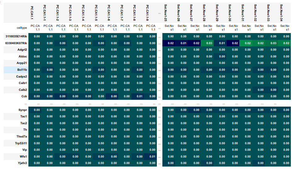
The AnnData object is added to sdata as a ScanpyDataFrame object, that strips away expresson information of genes that are absent in sdata. Per default, plankton expects cell type information to be stored under AnnData.obs.celltype, but a different label can be passed during object initialization.
This enables plankton to generate an expression signature matrix that’s stored at sdata.scanpy.signatures. The ScanpyDataFrape object also posesses a stats field with an identical format to the basic sdata.stats from tutorial 1.
A first handy step of quality control is to compare molecule count distributions in the two data modalities. Planton provides the function pl.hbar_compare for an interpretable visual representation of two stats objects:
pd.hbar_compare(sdata.stats,
                sdata.scanpy.stats,
                labels=['ISS','scRNAseq']
                )
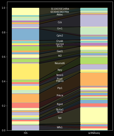
As the most significant result, the count comparison reveals an overabundance of Neurod6, and Cpls2 and an underabundance of Cck and Sst in the spatial data set.
We can plot the four molecules to reveal their spatial build-up:
misrepresented=['Neurod6','Cck','Cplx2','Sst']

plt.title('Celltypes with large intermodal count ratio differences')

sdata[sdata.g.isin(misrepresented)].scatter(legend=True,marker='x')
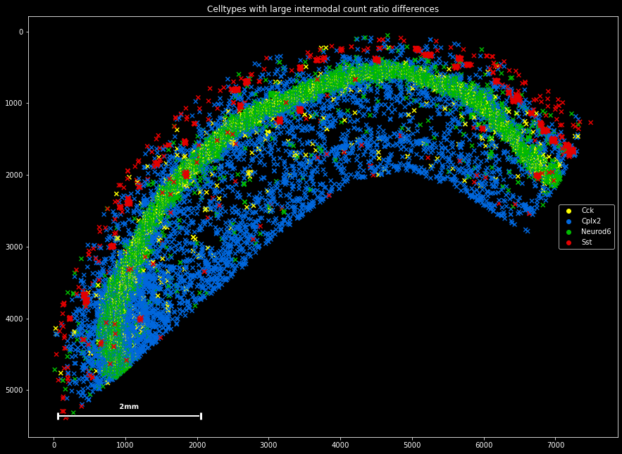
It seems that the overrepresented Neurod2 and the underrepresented Cck are both expressed mainly in the tightly packed pyramidal layer, whereas the overrepresented Cplx2 and the underrepresented Sst are mainly expressed by interneurons in the periphery. For now, we should accept this observation of different gene count distributions, as we cannot say whether the underlying mechanism is biological or methodological.
Such differences in gene count distributions across transcriptomics data modalities seems to re-occur across studies, and investigating the underlying mechanisms and dynamics would probably constitute an interesting research project by itself. In our case, it means that we might want to be careful when making claims about expression patterns amongst the four diverging genes. In my subjective experience, however, the signal in this sample seems comparatively stable compared to other available spot-based spatial transcriptomics data sets.
Plankton offers another feature to integrate single-cell and spatial transcriptomics data: It contains a simplified version of the SSAM algorithm by Park et al (2021) to generate preliminary cell type maps.
from plankton.utils import ssam
signatures = sdata.scanpy.generate_signatures()
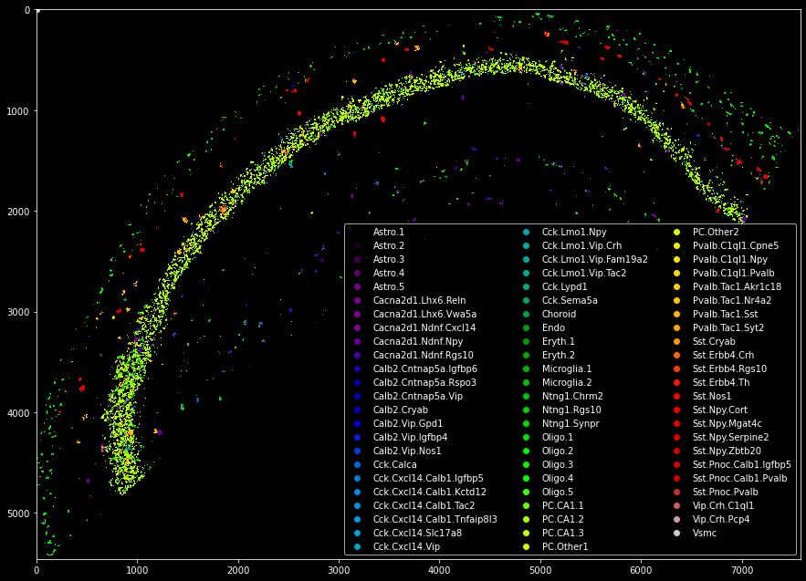
celltype_map = utils.ssam(sdata,signatures.T,kernel_bandwidth=5)
from matplotlib import cm

cmap = cm.get_cmap('nipy_spectral')
handlers = [plt.scatter([0],[0],color=cmap(f)) for f in np.linspace(0,1,len(sdata.scanpy.signature_matrix.index))]
plt.legend(handlers,sdata.scanpy.signature_matrix.index,ncol=3,loc='lower right')

plt.imshow(celltype_map,cmap='nipy_spectral',interpolation='none')