Tutorial 1: Data handling

Welcome to plankton’s tutorial series!

In this first part, you will learn how to create a SpatialData object, planktons core data handling device. You will learn the basics of data manipulation and get an introduction to plankton’s interactive analysis approach.

Data Preparation

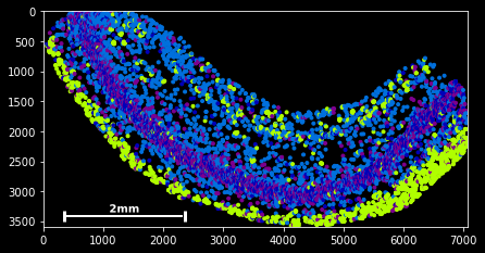
You will need a data set in order to see plankton in action. For this tutorial, we will use Xiaoyan Qian’s beautiful ISS scans of interneurons from the murine Hippocamupus from her 2018 publication. The data set contains 42580 detected molecule spots from 96 different gene classe, which is a relatively moderate size for the sake of this tutorial.

Activate the conda environment created during the Installation process and open the notebook plankton/tutorials/data-handling.ipynb. Running the first two cells should reformat the notebook layout and load the ISS data into memory. And we’re ready to go exploring!

Creating a SpatialData object

The SpatialData class inherits from pandas’s powerful DataFrame implementation and shares much of its functionality. In its most basic form, SpatialData has three input parameters, all of which expect a list with one entry per detected spot: genes containing the spots’ gene names (as strings) and x_coordinates/ y_coordinates containing the spots’ detected positions in micrometers.

Using the ISS-hippocampus data that was loaded into the notebook as a pandas DataFrame, a SpatialData initialisation would look like this:

import plankton as pl

sdata = pl.SpatialData(genes=xiaoyan_et_al.gene,
                       x_coordinates=xiaoyan_et_al.spotX,
                       y_coordinates=xiaoyan_et_al.spotY,)

This has created the object sdata, which is ready to be used for data exploration, manipulation and analysis!

just typing sdata into a jupyter cell and executing renders a short HTML overview of sdata:

sdata

	g	x	y	gene_id
0	Crym	534	3	23
1	Nrn1	563	3	51
2	Slc24a2	574	3	80
3	Gad1	22	540	32
4	Gad1	24	538	32
...	...	...	...	...
42575	Npy	6883	1974	48
42576	Npy	6889	1958	48
42577	Npy	6911	2433	48
42578	Npy	6940	2360	48
42579	Npy	6966	2257	48

_

We can see that the raw sdata table contains five columns: The first index column contains a unique index number for each data spot which remains constant throughout the analysis. g contains the spots’ gene label, x and y their spatial coordinates, and gene_ids an indexing integer that points g back to sdata’s list of gene classes.

Counts & statistics

As you can see from the sdata’s index, I did not lie about the total molecule count. So how about the gene count? Luckily, sdata has a field sdata.stats that contains basic gene-centric statistical information about the object. It is also implemented as a pandas DataFrame:

sdata.stats

	counts	count_ranks	count_indices	gene_ids
3110035E14Rik	2367	92	94	0
6330403K07Rik	442	65	20	1
Adgrl2	166	58	13	2
Aldoc	1343	89	79	3
Arpp21	528	69	54	4
...	...	...	...	...
Trp53i11	141	54	10	91
Vip	62	39	0	92
Wfs1	1734	90	59	93
Yjefn3	1	0	18	94
Zcchc12	56	36	45	95

It contains the series of gene classes (also accessible via sdata.genes) and gene counts (sdata.counts) alongside a few other statistical indices. This is also where the gene_ids are defined that we encountered earlier. We can see now that gene_ids can be used to map gene-wise information onto our spot data via indexing: sdata.genes[sdata.gene_ids], for example, returns the molecule-wise gene labels (and should hence be identical to sdata.g). Feel free to try it out!

Basic visualization

Easy and versatile hypothesis testing is vital for an interactive data analysis and modeling workflow, Luckily, spatial methods in the way we treat them are comparatively easy to visualize and illustrate! And people always appreciate a nice and colorful picture : )

SpatialData objects provide a simple scatter method for plotting spatial data:

sdata.scatter()

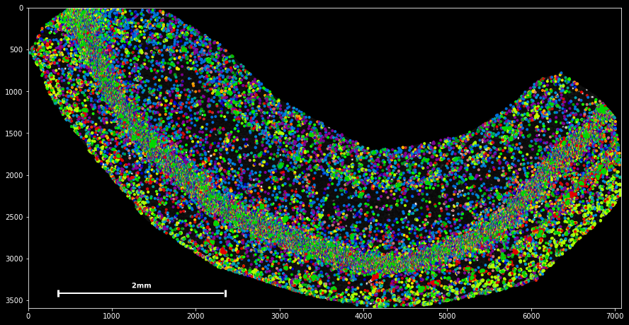
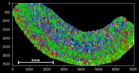
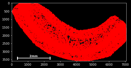
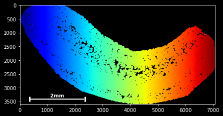
sdata.scatter is build on matplotlib’s scatter function, with which it shares the same keyword/argument structure:

sdata.scatter(color='r') 

sdata.scatter(marker='x') 

sdata.scatter(alpha=0.05) 

sdata.scatter(c=sdata.x) 

Thus, scatter provides an easy way to visualize how certain features are spatially distributed over the data points. The magic command %matplotlib notebook (executed on top of a cell) creates a panning and zooming function that allows closer data investigation. If the notebook mode becomes too fancy, you can always return to the default by executing %matplotlib inline.

Spatial or not: Data Indexing

The last basic feature for data handling is plankton’s indexing functionality. It slightly deviates from standard pandas indexing in that it always applied along the vertical axis first. Standard slicing notation [start:stop:step] is supported as well as boolean indexing and integer arrays.

The sdata.g.isin method is handy to subset the data points by comparison to a gene list. Furthermore, sdata.spatial provides a spatial view of the data set where slicing happens in the spatial domain and returns all data points located between the provided limits.

All slicing operations return a new SpatialData object, which we can use to create a single line plotting command:

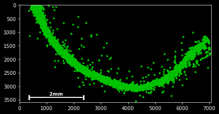
#slice - every 100th spot:
sdata[::100].scatter()

#boolean indexing for Neurod6
sdata[sdata.g=='Neurod6'].scatter()

#boolean indexing, multiple genes
genes=['Wfs1', 'Plp1', 'Cplx2',]
sdata[sdata.g.isin(genes)].scatter()

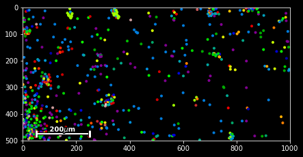
#spatial indexing
sdata.spatial[1000:2000,500:1000].scatter()

This should have you covered with the very basics of the available slicing functionality for spatial data frames.

---

Before we move on to an actual dataset analysis, here’s a final excercise to combine your newly acquired knowledge of sdata, sdata.stats, plotting and indexing:

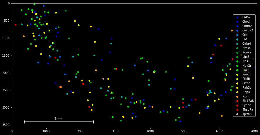
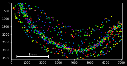
excercise

Try to plot all genes that occur less than 20 times in the data set. Increase the plot marker size to 100 and pass the argument legend=True to the plotting function. It should be possible in a single line of code.

---

solution:

• We learned that sdata.counts contains a list of count data for all genes.

• Hence, sdata.counts<20 returns a boolean array, indicating for each gene whether the count is below or above 20.

• As we learned during the `stats`_ section, we can project gene-centric information onto the whole data set by indexing with [sdata.gene_id]

• sdata.scatter takes the same arguments as its matplotlib equivalent, so the marker size is defined by the parameter s.

So, the solution is:

sdata[(sdata.counts<20)[sdata.gene_ids]].scatter(s=100,legend=True)